Notes on the Foundations of Reinforcement Learning and LLM Post-Training (Part 1)

Table of Contents
A Few Words Before We Begin
Reinforcement learning (RL) has recently emerged as one of the key techniques behind the post-training of large language models (LLMs) and vision-language models (VLMs). As I began reading more about methods such as PPO, RLHF, and GRPO, I realized that I often understood each idea separately but still struggled to see how they were connected. Some of the mathematical details were also quite difficult for me at first, and I found myself returning to the same concepts many times before they started to make sense.
I began writing these notes simply to organize what I was learning in my own words. They start from the basic ideas of reinforcement learning and gradually move toward their use in modern LLM post-training. I am sharing them here in the hope that they may be useful to someone else who is also trying to make sense of these concepts.
These are personal learning notes, so they may still contain mistakes, unclear explanations, or missing details. I am still learning as well :) If you notice anything that is incorrect or have suggestions for improving these notes, I would genuinely appreciate hearing from you.
How to Read These Notes
This post follows the path from basic RL concepts to PPO: concepts → policy gradients → REINFORCE → actor–critic → TRPO → PPO. Familiarity with probability, derivatives, and neural networks will help with the equations. You can read the intuition first and return to the derivations later.
Part 2 connects these ideas to language-model training, RLHF, and GRPO.
1. RL Concepts and Notation
What Problem Does RL Address?
In supervised learning, a model learns to predict outputs from examples. Reinforcement learning focuses on sequential decisions: an action changes the environment and affects the rewards available later. The goal is to learn a policy that maximizes cumulative reward through interaction.
The Agent–Environment Loop
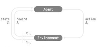
The agent interacts with an environment. At step $t$, it is in state $s_t \in \mathcal{S}$ and selects an action $a_t \in \mathcal{A}$. The environment produces a reward $r_t$ and a new state, according to the transition distribution $P(s_{t+1}\mid s_t,a_t)$. This transition model may be known or unknown to the agent.
One interaction cycle has three steps:
- Observe: receive the current state or observation.
- Act: select an action according to the policy.
- Receive feedback: observe the reward and the next state.
The cycle continues until the episode ends or the interaction is stopped. The agent’s objective is to improve its decisions based on the return across these interactions.
Supervised Learning vs. Reinforcement Learning
A supervised learning objective typically averages a prediction loss over a fixed dataset.

An RL objective averages return over trajectories generated by a policy. Changing the policy can also change which states and actions appear in the data.

| Aspect | Supervised learning | Reinforcement learning |
|---|---|---|
| Objective | Minimize prediction loss | Maximize expected return |
| Feedback | Targets or labels | Rewards, which may be delayed |
| Data | Often a fixed dataset | Often collected through interaction |
| Decisions | Predict an output | Choose actions with future consequences |
These describe common settings; offline RL, for example, also learns from a fixed dataset.
Key Concepts and Notation
States & Observations
- State ($s$): Information sufficient to describe the environment for predicting the next transition and reward, given an action.
- Observation ($o$): The information available to the agent, which may reveal all or only part of the state.
Fully Observed vs. Partially Observed: If the agent sees the full state $s$, the environment is fully observed. If it only sees an observation $o$, it’s partially observed.
- Representation: In deep RL, states and observations are typically represented as real-valued vectors, matrices, or tensors.
- Minor Notes on Notation: The symbol for state, $s$, is often used in formulas (e.g., $\pi(a|s)$) even when the agent practically only has access to an observation, $o$.
Action Spaces
- Action Space ($\mathcal{A}$): The set of all valid actions an agent can take in an environment.
- Discrete Action Space: A finite or countable set of actions, such as the legal moves in chess or Go.
- Continuous Action Space: Actions are represented by real-valued vectors. For example, the amount of torque to apply to a robot’s motors.
Policy
- Policy ($\pi$): A rule the agent uses to decide which action to take. It’s the agent’s “brain.”
Parameterized Policy: A policy whose behavior is defined by a function with adjustable parameters, $\theta$ (like the weights of a neural network). We can change the agent’s behavior by optimizing these parameters. Notation: $\pi_{\theta}(a|s)$ or $\mu_{\theta}(s)$.
- Deterministic Policy: The policy maps a state directly to a single action. Notation: $a_t = \mu_{\theta}(s_t)$
- Stochastic Policy: The policy outputs a probability distribution over actions.
- Notation: $a_t \sim \pi_{\theta}(\cdot | s_t)$
- Categorical Policy: Used for discrete action spaces. It’s like a classifier that outputs the probability for each possible action.
- Log-Likelihood: $\log \pi_{\theta}(a|s) = \log \left[P_{\theta}(s)\right]_a$, where $P_{\theta}(s)$ is the vector of action probabilities.
Diagonal Gaussian Policy: Used for continuous action spaces. The policy outputs a mean $\mu_{\theta}(s)$ and a standard deviation $\sigma_{\theta}(s)$ for a Gaussian distribution.
Sampling an Action: $a = \mu_{\theta}(s) + \sigma_{\theta}(s) \odot z$, where $z \sim \mathcal{N}(0, I)$ is a vector of standard normal noise and $\odot$ is an element-wise product.
- Log-Likelihood: For a $k$-dimensional action $a$:
Trajectories
- A sequence of states and actions in the world:
- The first state $s_0$ is sampled from the start-state distribution, sometimes denoted by $p_0$.
- State transitions are determined by the environment.
- Deterministic: $s_{t+1} = f(s_t, a_t)$
- Stochastic: $s_{t+1} \sim P(\cdot|s_t, a_t)$
- Trajectories are also frequently called episodes or rollouts.
Rewards and Return
- Reward ($r_t$): A scalar feedback signal indicating how well the agent is doing at a given step.
- Reward Function ($R$): Defines the reward, e.g., $r_t = R(s_t, a_t, s_{t+1})$.
- Return ($R(\tau)$): The cumulative reward over a trajectory.
- Finite-Horizon Undiscounted Return: The simple sum of rewards over a fixed number of $T$ steps.
Infinite-Horizon Discounted Return: A sum of all future rewards, discounted by a factor $\gamma \in (0,1)$. This makes rewards in the distant future less valuable than immediate rewards and helps ensure the sum converges.
RL Problem Formulation
- Objective: To find a policy $\pi$ that maximizes the expected return.
- Expected Return ($J(\pi)$): The expected return when the agent follows policy $\pi$. This requires averaging over all possible trajectories that could be sampled under $\pi$.
- Optimization Problem: Find the optimal policy, $\pi^*$, that yields the maximum possible expected return.
Value Function
Value functions estimate the expected return from a given state or state-action pair.
On-Policy Value Function ($V^{\pi}(s)$): The expected return if you start in state $s$ and follow policy $\pi$ forever. $V^{\pi}(s) = \underset{\tau \sim \pi}{\mathbb{E}} \left[ R(\tau) \mid s_0 = s \right]$
On-Policy Action-Value Function ($Q^{\pi}(s,a)$): The expected return if you start in state $s$, take action $a$, and then follow policy $\pi$ forever. $Q^{\pi}(s, a) = \underset{\tau \sim \pi}{\mathbb{E}} \left[ R(\tau) \mid s_0 = s, a_0 = a \right]$
- Optimal Value Function ($V^*(s)$): The maximum possible expected return from state $s$, achieved by following the optimal policy $V^{*}(s) = \max_{\pi} V^{\pi}(s)$
Optimal Action-Value Function ($Q^*(s,a)$): The maximum expected return starting from $s$, taking action $a$, and then following the optimal policy forever. $Q^{*}(s, a) = \max_{\pi} Q^{\pi}(s, a)$
- Optimal Action: If you know $Q^*(s,a)$, you can find the optimal action by choosing the one with the highest value $a^{*}_s = \arg \max_{a}Q^{*}(s, a)$
- Bellman Equations: These are fundamental self-consistency equations. The value of a state is the immediate reward plus the discounted value of the next state.
On-Policy:
$$ V^{\pi}(s) = \underset{a \sim \pi, s'\sim P}{\mathbb{E}}[r(s,a) + \gamma V^{\pi}(s')] $$$$ Q^{\pi}(s,a) = \underset{s'\sim P}{\mathbb{E}}[r(s,a) + \gamma \underset{a'\sim \pi}{\mathbb{E}}[Q^{\pi}(s',a')]] $$Optimal:
$$ V^*(s) = \max_a \underset{s'\sim P}{\mathbb{E}}[r(s,a) + \gamma V^*(s')] $$$$ Q^*(s,a) = \underset{s'\sim P}{\mathbb{E}}[r(s,a) + \gamma \max_{a'} Q^*(s',a')] $$Advantage Function ($A^{\pi}(s,a)$): Measures how much better taking action $a$ is compared to the average action from policy $\pi$ in state $s$. It is crucial for many policy gradient algorithms
$$ A^{\pi}(s, a) = Q^{\pi}(s, a) - V^{\pi}(s) $$Notation Summary
Throughout these notes, $r_t$ is the reward received after action $a_t$, and $G_t$ is the return from that step onward. Some references instead call that reward $r_{t+1}$; the indexing convention differs, not the underlying idea.
$$ G_t = \sum_{k=0}^{\infty}\gamma^k r_{t+k} = r_t + \gamma G_{t+1}. $$| Symbol | Meaning |
|---|---|
| $s_t$, $a_t$, $r_t$ | State, action, and immediate reward at step $t$ |
| $\pi_\theta(a_t \mid s_t)$ | Policy parameterized by $\theta$ |
| $G_t$ | Discounted return from step $t$ |
| $V^\pi(s)$ | Expected return from state $s$ under policy $\pi$ |
| $Q^\pi(s,a)$ | Expected return after action $a$ in state $s$, then following $\pi$ |
| $A^\pi(s,a)$ | Advantage: $Q^\pi(s,a)-V^\pi(s)$ |
| $V^*(s)$, $Q^*(s,a)$ | Optimal state and action values |
| $\gamma$ | Discount factor |
The value functions are related by
$$ V^\pi(s)=\mathbb{E}_{a\sim\pi(\cdot\mid s)}[Q^\pi(s,a)]. $$RL Algorithm Categories
- Based on how to update: On-policy vs. Off-policy Learning
On-policy: The behavior policy (used to collect samples) and the target policy (used to update) are the same policy. For example, in SARSA, the update uses a five-tuple sampled using an $\epsilon$-greedy policy: $(s,a,r,s',a')$
Off-Policy: The behavior policy (used to collect samples) and the target policy (used to update) are not the same. For example, in Q-learning, the update uses four-tuples data $(s,a,r,s')$ and $a'$ is obtained via $a^*=\arg\max_{a\prime}Q(s\prime,a\prime)$, rather than sampled from the behavior policy.
- Based on the access to environment model: Model-based vs. Model-free
An environment model describes how the environment responds to actions.
- Model-based: Rely on the model of the environment; either the model is known or the algorithm learns it explicitly.
- Model-free: No dependency on the model during learning.
- Based on how the policy is learned:
- Value-based: Learn a value function and derive a policy from it, rather than learning a separately parameterized policy.
- Policy-based: Directly optimize a parameterized policy.
2. Policy Gradients
We want to optimize the parameters $\theta$ of a stochastic policy $\pi_\theta$. Write the objective as expected return over trajectories:
$$ J(\theta)=\mathbb{E}_{\tau\sim\pi_\theta}[R(\tau)]. $$A trajectory begins at a state drawn from the initial-state distribution $p_0$. Equivalently, $J(\theta)=\mathbb{E}_{s_0\sim p_0}[V^{\pi_\theta}(s_0)]$. The initial-state distribution should not be confused with the distribution of states visited later under the policy.
Using gradient ascent, we update the policy in a direction that increases this objective:
$$ \theta\leftarrow\theta+\alpha\nabla_\theta J(\theta). $$The challenge is finding a gradient estimator from sampled interactions, even when the environment’s transition model is unknown.
3. The Policy Gradient Theorem
From Return to a Computable Gradient
The policy affects both the actions chosen and the states visited. The policy gradient theorem lets us express the gradient without explicitly differentiating the state-visitation distribution.
For the finite-horizon, undiscounted case in this derivation, let $R(\tau)=\sum_{t=0}^{T-1}r_t$. The log-derivative identity is
$$ \nabla_\theta p_\theta(\tau) =p_\theta(\tau)\nabla_\theta\log p_\theta(\tau). $$If the environment dynamics do not depend on $\theta$, only the policy terms contribute to the trajectory log-probability gradient:
$$ \nabla_\theta\log p_\theta(\tau) =\sum_{t=0}^{T-1}\nabla_\theta\log\pi_\theta(a_t\mid s_t). $$Combining these identities gives
$$ \begin{aligned} \nabla_\theta J(\theta) &=\nabla_\theta\int p_\theta(\tau)R(\tau)\,d\tau\\ &=\mathbb{E}_{\tau\sim\pi_\theta}\left[ R(\tau)\sum_{t=0}^{T-1}\nabla_\theta\log\pi_\theta(a_t\mid s_t) \right]. \end{aligned} $$The useful pattern is a return signal multiplied by the gradient of the action’s log-probability. We can estimate the expectation with sampled trajectories. See Spinning Up’s policy optimization derivation for the full argument.
Reward-to-Go and Action Values
Rewards received before an action do not help evaluate that action. We can instead use its reward-to-go, $G_t=\sum_{k=t}^{T-1}r_k$ in this undiscounted derivation:
$$ \nabla_\theta J(\theta) =\mathbb{E}_{\tau\sim\pi_\theta}\left[ \sum_{t=0}^{T-1}G_t\nabla_\theta\log\pi_\theta(a_t\mid s_t) \right]. $$Conditioning on $(s_t,a_t)$ replaces $G_t$ with its expectation, $Q^\pi(s_t,a_t)$. This connects the trajectory estimator to the action-value form of the policy gradient. In a discounted objective, the corresponding time weights must also be included consistently.
Why Variance Matters
Bias is systematic error: an unbiased estimator equals the target gradient on average. Variance describes how much the estimate changes across sampled batches.
Monte Carlo policy-gradient estimates can be unbiased while still having high variance. Different trajectories can produce very different returns, so a small batch may give a noisy update. The next sections introduce baselines and learned value functions to make that signal more useful.
4. REINFORCE and Baselines
Intuition
REINFORCE estimates the policy gradient using complete episodes. For each action, it uses the observed return from that point onward as a Monte Carlo estimate of the action value.
$$ \mathbb{E}[G_t\mid s_t,a_t]=Q^\pi(s_t,a_t). $$This avoids learning a critic, but the return depends on all the later transitions and rewards. That is the source of its noisy updates.
Algorithm
Choose a learning rate $\alpha$, discount factor $\gamma$, and number of episodes. Initialize the policy parameters $\theta$.
- Collect a complete episode. Sample actions from the policy and store states, actions, and rewards.
- Compute returns backward. Start with $G=0$ and apply $G\leftarrow r_t+\gamma G$ from the final step to the first.
- Accumulate the policy gradient. Weight each action’s log-probability gradient by its return.
- Update the policy. Take a gradient-ascent step, then collect fresh data.
For the discounted start-state objective, an episode estimate is
$$ \hat g=\sum_{t=0}^{T-1}\gamma^tG_t\nabla_\theta\log\pi_\theta(a_t\mid s_t), \qquad \theta\leftarrow\theta+\alpha\hat g. $$Setting $\gamma=1$ recovers the undiscounted estimator above. The following is pseudocode, with environment and policy operations left abstract:
initialize policy parameters theta
repeat for each episode:
    collect states, actions, rewards using the current policy
    G = 0
    returns = an array with one entry per action
    for t from T - 1 down to 0:
        G = rewards[t] + gamma * G
        returns[t] = G
    gradient = 0
    for t from 0 to T - 1:
        gradient += gamma**t * returns[t] * grad_log_policy(actions[t], states[t])
    theta += learning_rate * gradient
Choosing the Weight on the Policy Gradient
The general pattern is a score-function gradient multiplied by a weight $\psi_t$. Several choices connect REINFORCE to actor–critic methods:
- Whole-trajectory return: every action receives the same trajectory-level signal.
- Reward-to-go $G_t$: each action receives only the rewards from that step onward.
- Baseline-adjusted return $G_t-b(s_t)$: subtract a state-dependent baseline to reduce variance without changing the expected policy gradient.
- Action value $Q^\pi(s_t,a_t)$: use the expected return conditioned on the state and action.
- Advantage $A^\pi(s_t,a_t)$: subtract $V^\pi(s_t)$ from the action value to compare an action with the policy’s average behavior in that state.
- TD-based advantage estimate: use a learned critic and observed transitions, as described next.
A useful baseline should explain variation in return without depending on the sampled action. Its purpose is to improve the gradient estimate, rather than change which policy we want to learn.
5. Actor–Critic Methods
Motivation and Intuition
An actor learns the policy, while a critic learns a value function that helps evaluate the actor’s decisions. Instead of waiting for a complete Monte Carlo return, we can combine an observed reward with the critic’s prediction of what happens next.
The actor has parameters $\theta$ and policy $\pi_\theta(a\mid s)$. Here the critic has parameters $w$ and predicts $V_w(s)$. Other actor–critic algorithms may learn an action-value function instead.
From the Bellman Equation to a TD Error
Recall the relationship between action values and state values:
$$ Q^\pi(s,a)=\mathbb{E}_{r,s'\mid s,a}[r+\gamma V^\pi(s')]. $$For a sampled transition, the one-step target and temporal-difference (TD) error are
$$ y_t=r_t+\gamma(1-d_t)V_w(s_{t+1}), \qquad \delta_t=y_t-V_w(s_t), $$where $d_t=1$ at a terminal state and $0$ otherwise. The terminal mask prevents bootstrapping beyond the end of an episode.
With an exact value function, the conditional expectation of this TD error is the advantage. A sampled transition remains noisy, and an imperfect learned value function can introduce bias. Stochastic transitions alone do not make the conditional estimate biased.
Updating the Actor and Critic
The actor uses $\delta_t$ as an advantage estimate. A per-transition update direction is
$$ \hat g_t=\delta_t\nabla_\theta\log\pi_\theta(a_t\mid s_t). $$A positive TD error encourages the sampled action; a negative one discourages it. The critic minimizes a squared prediction error:
$$ \mathcal{L}_V(w)=\frac12\left(V_w(s_t)-\operatorname{stopgrad}(y_t)\right)^2. $$Holding the target fixed gives
$$ \nabla_w\mathcal{L}_V(w)=-\delta_t\nabla_wV_w(s_t). $$Consequently, gradient descent on this loss updates $w$ in the direction $+\delta_t\nabla_wV_w(s_t)$. Keeping the loss gradient and the parameter-update direction separate makes the sign easier to follow.
Algorithm and Implementation Notes
- Act: sample $a_t\sim\pi_\theta(\cdot\mid s_t)$.
- Observe: receive $r_t$, $s_{t+1}$, and the terminal flag.
- Evaluate: compute the target $y_t$ and TD error $\delta_t$.
- Update the critic: minimize the value prediction loss with the target held fixed.
- Update the actor: use the detached TD error to weight the log-probability gradient.
In PyTorch, .detach() stops gradients through a tensor. For the critic, detach the bootstrap target; for the actor, detach the advantage estimate so that the actor loss does not also optimize the critic through that weight.
Implementations often collect a small batch of transitions before updating. Batch size and rollout length affect the trade-off between noisy estimates and delayed updates.
6. Trust Region Policy Optimization (TRPO)
Why Limit the Policy Update?
This section provides background for PPO rather than a full TRPO derivation. A large parameter update can change a neural-network policy substantially and reduce its performance. TRPO uses a trust region to limit the change while improving an advantage-based surrogate objective.
We collect data with an old policy $\pi_{\mathrm{old}}$, then evaluate candidate policies against the old policy’s advantages. Keeping that reference fixed is essential: the expected advantage of a policy under its own action distribution is zero.
The Surrogate Objective and Constraint
Define $d_{\mathrm{old}}$ as the state-visitation distribution used by the surrogate and $\rho_\theta(s,a)=\pi_\theta(a\mid s)/\pi_{\mathrm{old}}(a\mid s)$. The practical TRPO optimization problem combines an advantage-weighted objective with an average KL constraint:
$$ \begin{aligned} \max_\theta\quad & \mathbb{E}_{s\sim d_{\mathrm{old}},\,a\sim\pi_{\mathrm{old}}} \left[\rho_\theta(s,a)A^{\pi_{\mathrm{old}}}(s,a)\right]\\ \text{subject to}\quad & \mathbb{E}_{s\sim d_{\mathrm{old}}}\left[ D_{\mathrm{KL}}\left(\pi_{\mathrm{old}}(\cdot\mid s)\,\|\,\pi_\theta(\cdot\mid s)\right) \right]\leq\delta. \end{aligned} $$The importance weight adjusts an action’s contribution according to how likely the candidate policy is to choose it relative to the rollout policy. For a positive advantage, increasing the ratio increases its contribution to the surrogate; decreasing the ratio reduces that contribution. Negative advantages reverse the preference.
The KL constraint limits the average distributional change over the sampled states. The threshold $\delta$ controls the size of the trust region. This helps keep the local surrogate useful as the policy changes; it is not a guarantee that every individual state or action changes by a fixed amount.
See the TRPO explanation in Spinning Up and the original paper for the optimization procedure.
Why Importance Sampling?
Suppose we want an expectation under a target distribution $p$, but our samples come from $q$. If $q(x)>0$ wherever $p(x)>0$, we can rewrite
$$ \begin{aligned} \mathbb{E}_{x\sim p}[h(x)] &=\int h(x)p(x)\,dx\\ &=\int h(x)\frac{p(x)}{q(x)}q(x)\,dx\\ &=\mathbb{E}_{x\sim q}\left[\frac{p(x)}{q(x)}h(x)\right]. \end{aligned} $$In the policy surrogate, the ratio reweights actions from the old policy. The surrogate still uses the old state distribution, so it should not be mistaken for an exact evaluation of the candidate policy’s full return.
This is also useful background for PPO: collect a rollout batch, save its action log-probabilities, and optimize a surrogate over several passes through that batch. As the policy moves away from the rollout policy, the approximation becomes less reliable. Policy-change controls help address that problem.
7. Proximal Policy Optimization (PPO)
The Clipped Surrogate Objective
TRPO solves a constrained optimization problem. PPO-Clip uses a simpler clipped surrogate objective that can be optimized with ordinary gradient-based updates.
Define the new-to-old probability ratio as
$$ \rho_t(\theta)=\frac{\pi_\theta(a_t\mid s_t)}{\pi_{\mathrm{old}}(a_t\mid s_t)}. $$The old policy is the policy that collected the rollout. Let $\hat A_t$ be an advantage estimate computed from that rollout. PPO maximizes
$$ L^{\mathrm{CLIP}}(\theta)=\mathbb{E}_t\left[ \min\left(\rho_t(\theta)\hat A_t, \operatorname{clip}(\rho_t(\theta),1-\epsilon,1+\epsilon)\hat A_t\right) \right]. $$Clipping removes the incentive for certain changes that move the probability ratio too far in a favorable direction. It does not enforce a hard bound on the actual ratio or guarantee a small KL divergence. See Spinning Up’s PPO explanation.
Here I use $\rho_t$ for the probability ratio so it is visually distinct from the reward $r_t$.
Generalized Advantage Estimation (GAE)
The advantage tells us how much better an action is than the policy’s average behavior in that state. Two ways to estimate it are:
- Monte Carlo: use the full observed return minus a baseline. This avoids bootstrapping at an episode’s end, but may have high variance.
- One-step TD: combine an immediate reward with the critic’s next-state estimate. This often reduces variance but depends on the accuracy of the critic.
GAE interpolates between these approaches. For readability, the equations below omit terminal masks; at episode boundaries, stop bootstrapping and truncate the sums appropriately.
Start with the TD error $\delta_t=r_t+\gamma V(s_{t+1})-V(s_t)$. Multi-step estimates are
$$ \begin{aligned} \hat A_t^{(1)}&=\delta_t,\\ \hat A_t^{(2)}&=\delta_t+\gamma\delta_{t+1},\\ \hat A_t^{(3)}&=\delta_t+\gamma\delta_{t+1}+\gamma^2\delta_{t+2},\\ \hat A_t^{(k)}&=\sum_{i=0}^{k-1}\gamma^i\delta_{t+i}. \end{aligned} $$Expanding the TD errors makes the intermediate value terms cancel:
$$ \hat A_t^{(k)} =-V(s_t)+\sum_{i=0}^{k-1}\gamma^i r_{t+i}+\gamma^kV(s_{t+k}). $$For $0\leq\lambda\lt 1$, an exponentially weighted average gives
$$ \begin{aligned} \hat A_t^{\mathrm{GAE}} &=(1-\lambda)\sum_{k=1}^{\infty}\lambda^{k-1}\hat A_t^{(k)}\\ &=(1-\lambda)\sum_{k=1}^{\infty}\lambda^{k-1} \sum_{l=0}^{k-1}\gamma^l\delta_{t+l}\\ &=\sum_{l=0}^{\infty}\gamma^l\delta_{t+l} \left[(1-\lambda)\sum_{k=l+1}^{\infty}\lambda^{k-1}\right]\\ &=\sum_{l=0}^{\infty}(\gamma\lambda)^l\delta_{t+l}. \end{aligned} $$The parameter $\lambda$ controls the trade-off:
- At $\lambda=0$, GAE reduces to the one-step TD error.
- At $\lambda=1$, the finite-episode sum reduces to the Monte Carlo return minus the baseline when the terminal value is zero.
- Intermediate values trade reliance on long sampled returns against reliance on learned value estimates.
The GAE paper develops this bias–variance perspective in more detail.
Entropy Bonus
An entropy bonus encourages exploration by discouraging the policy from becoming too concentrated too early. Without sufficient exploration, the agent may commit to a suboptimal action before discovering alternatives.
Formula:
$$ S[\pi_\theta](s_t) = H(\theta) = - \mathbb{E}_{a_t} [\log \pi_\theta (a_t | s_t)] = -\sum_a\pi_\theta (a | s_t) \log \pi_\theta (a | s_t) $$For categorical logits, the following PyTorch snippet computes the entropy. It assumes logits_current contains valid, unpadded positions:
import torch.nn.functional as F

# Compute entropy of current policy
probs_current = F.softmax(logits_current, dim=-1)
log_probs_current = F.log_softmax(logits_current, dim=-1)
entropy = -(probs_current * log_probs_current).sum(dim=-1)
# Average over sequence and batch
entropy_bonus = entropy.mean()
Training the Value Function
PPO also fits a critic. Let $V_w$ be the current value function and let $\hat V_t$ be a return target computed from the rollout. With GAE, a common target is
$$ \hat V_t=\hat A_t^{\mathrm{GAE}}+V_{w_{\mathrm{old}}}(s_t). $$This is a bootstrapped return target; it is not generally identical to the observed Monte Carlo return. Fit the critic with the target held fixed:
$$ \mathcal{L}^{\mathrm{VF}}_t(w) =\frac12\left(V_w(s_t)-\operatorname{stopgrad}(\hat V_t)\right)^2. $$Average the loss over the batch. The actor and critic may use separate networks or share a backbone with different output heads. Here, $\theta$ and $w$ distinguish the policy and value parameters even when discussing their losses together.
The Combined PPO Objective
One common combined objective is maximized:
$$ J_{\mathrm{PPO}}(\theta,w) =\mathbb{E}_t\left[ L_t^{\mathrm{CLIP}}(\theta) -c_1\mathcal{L}_t^{\mathrm{VF}}(w) +c_2H(\pi_\theta(\cdot\mid s_t)) \right]. $$A loss minimized by an optimizer has the opposite sign. The clipped term updates the actor, the value loss trains the critic, and the entropy term encourages exploration.
| Parameter | Role |
|---|---|
| $\gamma$ | Discounting future rewards |
| $\lambda$ | GAE’s bias–variance trade-off |
| $\epsilon$ | Clipping threshold in the surrogate objective |
| $c_1$ | Weight of the value loss |
| $c_2$ | Weight of the entropy bonus |
Key Takeaways
- Policy gradients connect sampled rewards to changes in action probabilities.
- REINFORCE uses complete returns; a baseline can reduce variance.
- Actor–critic methods learn value estimates to guide policy updates.
- TRPO constrains policy change, while PPO uses a clipped surrogate.
- GAE, value targets, and entropy each address a different part of training.
Continue with Part 2, which covers RL in the LLM/VLM setting, RLHF, the full PPO training pipeline, and GRPO.
Acknowledgements
These notes would not have been possible without the many excellent books, lecture notes, blog posts, papers, and open-source resources created by the machine learning community. I am deeply grateful to all of the authors and educators whose work helped me understand reinforcement learning and LLM post-training. Many of the explanations and intuitions presented here were inspired by or built upon these resources, although any mistakes, misunderstandings, or inaccuracies are entirely my own.
If you are interested in learning more, I highly encourage you to explore the references below. They provide much deeper and more rigorous treatments than these personal notes and have been invaluable throughout my learning journey.
References
RL Foundations
Policy Gradient Papers
Sutton et al. — Policy Gradient Methods for Reinforcement Learning with Function Approximation
Mnih et al. — Asynchronous Methods for Deep Reinforcement Learning
RLHF
Christiano et al. — Deep Reinforcement Learning from Human Preferences
Ouyang et al. — Training Language Models to Follow Instructions with Human Feedback
Ziegler et al. — Fine-Tuning Language Models from Human Preferences
PPO and GRPO Explanations

Hi! I’m Chi, and I am interested in developing multimodal AI systems that can meaningfully improve medical understanding and support clinical decision-making.
My research lies at the intersection of machine learning and medical imaging, with a particular focus on multimodal foundation models, medical reasoning, and trustworthy AI for healthcare. I am especially interested in building clinically grounded and reliable models that can learn from complex medical data while remaining interpretable and useful in real-world settings.
During my research journey, I have been fortunate to work under the guidance of Prof. Yueming Jin at the National University of Singapore, Prof. Lee Hwee Kuan at the Bioinformatics Institute (A*STAR), Prof. Hieu Pham at VinUniversity, and Prof. Ravishankar K. Iyer at the University of Illinois Urbana–Champaign. Feel free to reach out if you would like to chat about medical AI, multimodal learning, or research in general!