Notes on the Foundations of Reinforcement Learning and LLM Post-Training (Part 2)

Table of Contents
Before We Begin
Part 1 introduces policy gradients, value functions, actor–critic methods, and PPO. Here, I connect those ideas to language-model post-training: how a response becomes a trajectory, how preferences become rewards, and how PPO and GRPO update the model.
The reading path is language generation as RL → preference learning → SFT and reward models → PPO training → GRPO. If the notation becomes unfamiliar, return to Part 1’s concepts and PPO sections.
1. Language Generation as an RL Problem
Problem Formulation
Given a prompt, a language model generates a response one token at a time. This autoregressive process gives us a concrete mapping to the RL concepts from Part 1.
| RL concept | Language-model interpretation |
|---|---|
| State $s_t$ | The prompt and all tokens generated so far |
| Action $a_t$ | The next token |
| Policy $\pi_\theta(a_t\mid s_t)$ | A probability distribution over the vocabulary |
| Transition | Append the selected token: $s_{t+1}=[s_t,a_t]$ |
| Reward $r_t$ | Feedback assigned after generating a token |
| Value $V(s_t)$ | Expected future return from the current prefix |
The initial state is the prompt. For a VLM, the conditioning context can also include visual input. The state transition is deterministic once the next token has been selected, even though token sampling is stochastic.
The Optimization Objective
Let $x$ denote a prompt and $y$ a response. With a response-level reward $r(x,y)$, the objective is
$$ \max_\theta\;\mathbb{E}_{x\sim D,\,y\sim\pi_\theta(\cdot\mid x)}[r(x,y)]. $$A KL penalty discourages the policy from drifting too far from a reference model. A regularized objective can be written as
$$ \max_\theta\;\mathbb{E}_{x\sim D}\left[ \mathbb{E}_{y\sim\pi_\theta(\cdot\mid x)}[r(x,y)] -\beta D_{\mathrm{KL}}\left(\pi_\theta(\cdot\mid x)\,\|\,\pi_{\mathrm{ref}}(\cdot\mid x)\right) \right]. $$Equivalently, using the sampled log-probability ratio inside the expectation:
$$ \max_\theta\;\mathbb{E}_{x\sim D,\,y\sim\pi_\theta(\cdot\mid x)}\left[ r(x,y)-\beta\log\frac{\pi_\theta(y\mid x)}{\pi_{\mathrm{ref}}(y\mid x)} \right]. $$Here $\beta$ controls the strength of the penalty. This fixed reference policy has a different role from the old rollout policy used in PPO’s clipping ratio.
2. Learning from Human Preferences
Why Learn a Reward Function?
For tasks such as conversation or summarization, it is difficult to write a reward function that captures what people want. Comparing examples can be easier than assigning an absolute numerical score. RLHF uses those comparisons to learn a reward model, then optimizes a policy against that model.
Preference Learning, Step by Step
1. Collect Preference Data
Annotators compare two segments of agent behavior, $\sigma^1$ and $\sigma^2$. A segment is a sequence of state–action pairs:
$$ \sigma^i=((s_0^i,a_0^i),\ldots,(s_{k-1}^i,a_{k-1}^i)). $$Use a target $p$ of $1$ when the first segment is preferred, $0$ when the second is preferred, and $0.5$ for a tie. This notation makes the label convention explicit.
2. Fit a Reward Model
The model assigns a score to each segment by summing predicted per-step rewards:
$$ S_{\hat r}(\sigma)=\sum_t\hat r(s_t,a_t). $$Under a Bradley–Terry preference model, the probability that the first segment is preferred is
$$ \hat P(\sigma^1\succ\sigma^2) =\frac{\exp S_{\hat r}(\sigma^1)} {\exp S_{\hat r}(\sigma^1)+\exp S_{\hat r}(\sigma^2)}. $$This is a softmax over two scores: a larger predicted cumulative reward gives a higher preference probability. The language-model example later uses a scalar score for a whole response rather than a sum of learned per-token rewards.
Let $\hat p=\hat P(\sigma^1\succ\sigma^2)$. Fit the predictions to the preference labels with cross-entropy:
$$ \mathcal{L}(\hat r) =-\mathbb{E}_{(\sigma^1,\sigma^2,p)\sim D} \left[p\log\hat p+(1-p)\log(1-\hat p)\right]. $$For strictly ordered pairs, denote the preferred segment by $\sigma^+$ and the rejected segment by $\sigma^-$. The loss becomes
$$ \begin{aligned} \mathcal{L}(\hat r) &=-\mathbb{E}\left[\log\hat P(\sigma^+\succ\sigma^-)\right]\\ &=-\mathbb{E}\left[ \log\frac{\exp S_{\hat r}(\sigma^+)} {\exp S_{\hat r}(\sigma^+)+\exp S_{\hat r}(\sigma^-)} \right]. \end{aligned} $$3. Optimize the Policy
Once the reward function is learned, an RL algorithm uses it as feedback:
- The policy generates a response or trajectory.
- The reward model assigns a score.
- A policy-optimization algorithm such as PPO uses the score to update the policy.
- The updated policy generates new samples for the next round.
The human-preference RL paper alternates preference collection, reward learning, and policy learning. Collecting new feedback can help cover behavior that was absent from earlier data, but human annotation is expensive. Automated preference labeling, including RLAIF, is another approach to obtaining feedback.
The learned reward remains a proxy for the preferences represented in its training data. Improving that score and improving behavior should be evaluated separately.
3. The Models in the RLHF Pipeline
The PPO-based pipeline discussed here has four roles: actor, critic, reward model, and reference model. The SFT checkpoint supplies an initial policy and commonly initializes other components.
| Component | Role during RL | Updated during this stage? |
|---|---|---|
| Actor / policy | Generates responses and learns from rewards | Yes |
| Critic / value model | Predicts returns for response prefixes | Yes |
| Reward model | Scores completed responses | Frozen in this setup |
| Reference model | Supplies a fixed distribution for the KL penalty | No |
The SFT model is a pretrained language model further trained on demonstrations. It provides a useful starting point before preference-based RL.
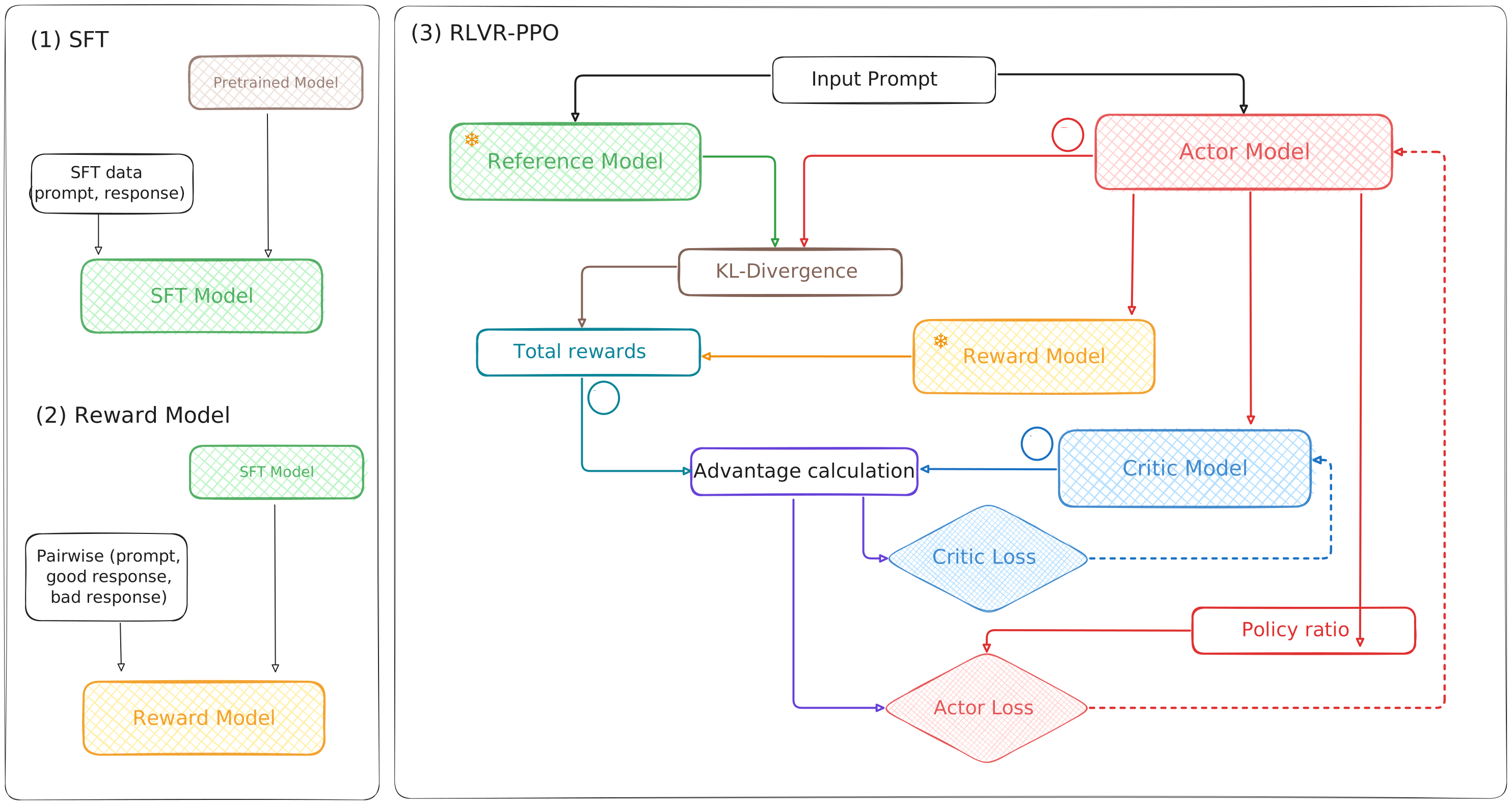
The overall sequence is:
- Prepare the SFT checkpoint using prompt–response demonstrations.
- Train the reward model using preferred and rejected response pairs.
- Generate rollouts with the actor and score the sampled tokens under the actor and reference policies.
- Build the reward signal from response scores and the KL penalty.
- Estimate advantages and return targets using rewards and critic predictions.
- Update actor and critic with their respective losses, then collect another rollout batch.
The InstructGPT paper is a primary reference for this style of language-model training pipeline.
4. SFT and Reward Model Training
Supervised Fine-Tuning (SFT)
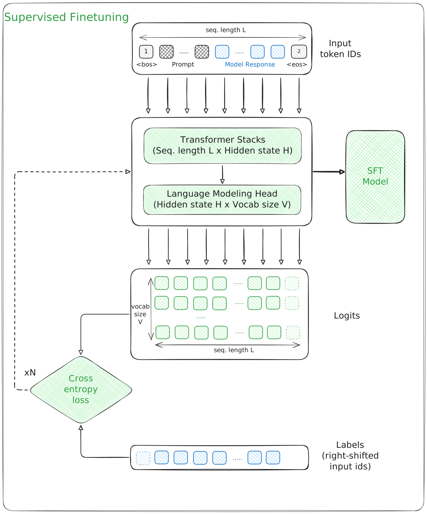
SFT trains the pretrained model on demonstration responses. The resulting checkpoint initializes the actor and the frozen reference policy in this setup.
Reward Model
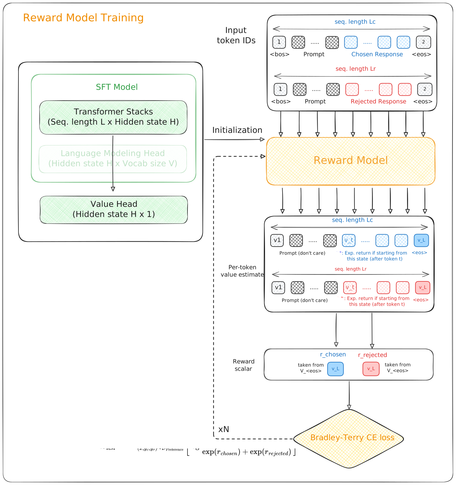
Train the reward model after SFT and before the PPO stage. Its input is a prompt–response pair, and its output is a scalar preference score.
Initialization
Initialize the reward model from the SFT checkpoint. Add a scalar reward head, usually a linear projection, to produce the response score:
$$ r (x,y) = \text{Linear}(h_\text{final token}) $$Preference Loss
Each preference example contains:
- $x$: the prompt
- $y_w$: the chosen (preferred) response
- $y_l$: the rejected (less preferred) response Train the model to assign a higher score to the preferred response. The pairwise loss is:
where $\sigma(x) = \frac{1}{1 + \exp(-x)}$ is a sigmoid function, hence the loss can be written as:
$$ \mathcal{L}_\text{RM}=-\mathbb{E}_{(x,y_w,y_l)\sim D}\left[\log\left(\frac{\exp(r(x,y_w))}{\exp(r(x,y_w))+\exp(r(x,y_l))}\right)\right] $$The following PyTorch class computes the pairwise loss, with an optional margin:
import torch.nn as nn
import torch.nn.functional as F

class PairWiseLoss(nn.Module):
    """Pairwise preference loss for a reward model."""

    def forward(self, chosen_reward, reject_reward, margin=None):
        reward_difference = chosen_reward - reject_reward
        if margin is not None:
            reward_difference = reward_difference - margin
        return -F.logsigmoid(reward_difference).mean()
Interpreting the Reward Output
In this setup, the reward model assigns a single scalar score $r(x,y)$ to a completed response. A common implementation applies a scalar head to the final token’s hidden representation. That representation depends on the preceding context, so the score can summarize the response rather than only its last token.
Other aggregation choices include sums, means, weighted sums, or attention-based pooling. The aggregation is an implementation choice; it should match how the reward model was trained.
5. PPO Training
Actor Model
The actor generates responses token by token and is the model being optimized during RL. It begins from the SFT checkpoint; the reward model is already trained and frozen.
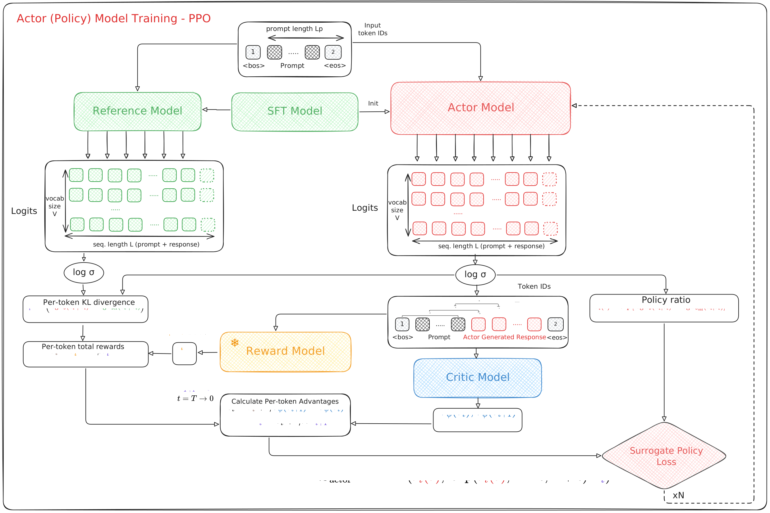
For each rollout batch:
- Generate responses. Sample token IDs from the actor’s output distribution and save their rollout log-probabilities.
- Score the responses. The reward model supplies response scores; the reference model supplies token log-probabilities for the KL penalty.
- Estimate values and advantages. The critic predicts values for prefixes, which combine with the rewards to produce GAE estimates.
- Optimize the actor. Recompute the current policy’s log-probabilities and compare them with the saved rollout probabilities.
Let $\pi_{\mathrm{old}}$ be the rollout policy and $\rho_t(\theta)=\pi_\theta(a_t\mid s_t)/\pi_{\mathrm{old}}(a_t\mid s_t)$. The per-token actor loss is
$$ \mathcal{L}_{\mathrm{actor},t} =-\min\left( \rho_t(\theta)\hat A_t, \operatorname{clip}(\rho_t(\theta),1-\epsilon,1+\epsilon)\hat A_t \right). $$The negative sign turns the objective from Part 1 into a loss to minimize. In practice, aggregate over valid response tokens and the batch, masking padding and prompt tokens as appropriate. Treat advantages and old log-probabilities as fixed targets during each update.
An entropy bonus can also be included. It is separate from the clipping term and from the reference-policy KL penalty.
Critic Model
The critic predicts expected future return from each prefix. It learns alongside the actor, but uses a value-prediction loss.
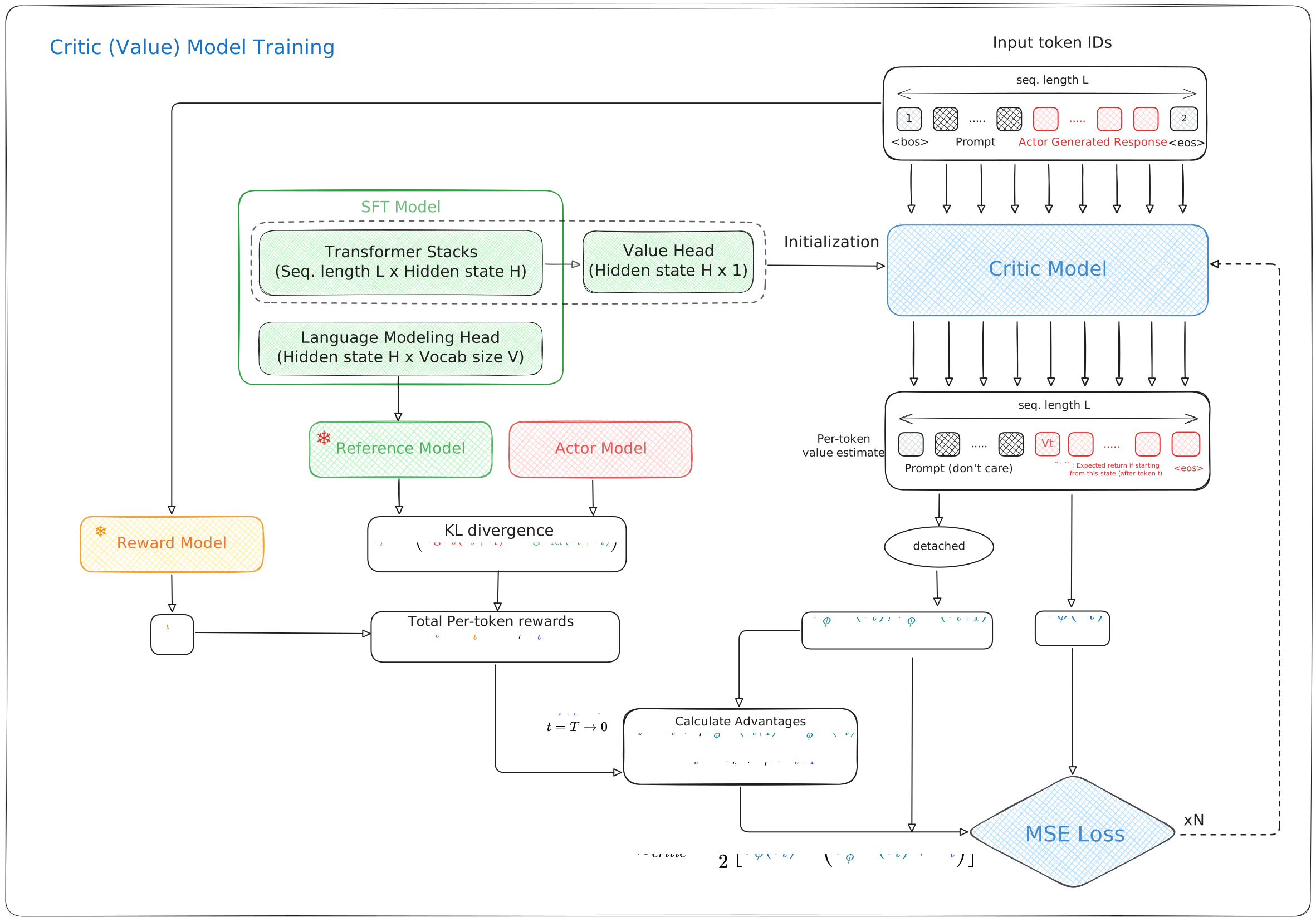
Initialization. Possible designs include an SFT-based model with a value head, initialization from the trained reward model, or a value head sharing a backbone with the actor. Separate actor and critic networks are one design choice, not a requirement of every PPO implementation.
TD errors and GAE. For rollout values $V_{w_{\mathrm{old}}}$, define
$$ \delta_t=r_t+\gamma(1-d_t)V_{w_{\mathrm{old}}}(s_{t+1}) -V_{w_{\mathrm{old}}}(s_t). $$Here $d_t$ indicates termination. The discount factor is $\gamma$; $\lambda$ instead controls the weighting of TD errors in GAE. For a rollout ending at $T$,
$$ \hat A_t^{\mathrm{GAE}}=\sum_{l=0}^{T-t}(\gamma\lambda)^l\delta_{t+l}, \qquad \hat V_t=\hat A_t^{\mathrm{GAE}}+V_{w_{\mathrm{old}}}(s_t). $$Stop the sum at episode boundaries and handle bootstrapping at nonterminal rollout cutoffs. The critic minimizes
$$ \mathcal{L}_{\mathrm{critic},t} =\frac12\left(V_w(s_t)-\operatorname{stopgrad}(\hat V_t)\right)^2. $$Using $\hat V_t$ for the return target avoids confusing it with the immediate reward $r_t$.
Reference Model and Token Rewards
The reference policy is usually a frozen copy of the SFT policy. It supplies a fixed point of comparison while the actor changes. By contrast, the old policy is refreshed when collecting new rollouts and supplies PPO’s probability-ratio denominator.
For a sampled token, the log-probability ratio is
$$ k_t=\log\pi_\theta(a_t\mid s_t)-\log\pi_{\mathrm{ref}}(a_t\mid s_t). $$Its expectation under $a_t\sim\pi_\theta(\cdot\mid s_t)$ is the forward KL divergence. A single sampled value is not the full KL divergence and can be negative.
For a response ending at token $T$, one common reward decomposition is
$$ r_t= \begin{cases} -\beta k_t, & t\lt T,\\ r(x,y)-\beta k_t, & t=T. \end{cases} $$Every token receives the KL shaping term, while the final token also receives the reward model’s response score. Equivalently,
$$ r_t=\mathbb{I}[t=T]\,r(x,y)-\beta k_t. $$The terminal reward is propagated to earlier tokens through the return and advantage estimates. During rollout processing, compute these quantities using the rollout policy and hold the resulting targets fixed for PPO updates.
Practical Training Considerations
These are useful implementation topics to revisit once the main pipeline is clear:
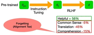
- Pretraining loss and alignment tax: monitor whether preference optimization reduces performance on other tasks, and consider how auxiliary training objectives affect that trade-off.
- KL reward scaling: choose and monitor the penalty coefficient $\beta$.
- Reward normalization: make the treatment of reward scale explicit.
- Advantage normalization: distinguish this from normalizing the raw reward.
- Learning rate: tune actor and critic optimization with their different objectives in mind.
Open Challenges
Two questions remain central: does the policy exploit weaknesses in the reward model (reward hacking), and do improvements transfer beyond the training prompts (generalization)? A higher training reward alone does not answer either question.
6. Group Relative Policy Optimization (GRPO)
Motivation
The PPO pipeline above requires an actor, a critic, a reward signal, and a reference policy. Running these components can be expensive, and the learned critic adds another estimate to fit and maintain.
DeepSeekMath introduces GRPO as a way to obtain an advantage signal from a group of responses to the same prompt, without a separate learned critic.
Which Component Changes?
- Actor: still generates responses and receives policy updates.
- Reward signal: still evaluates responses. Depending on the task, it can come from a model or a verifiable rule.
- Reference policy: remains in the original KL-regularized GRPO objective.
- Critic: replaced by a baseline derived from rewards within the sampled group.
The key change is how the advantage is estimated. It does not remove the need to evaluate the generated responses.
Advantage Function Estimation in GRPO
GRPO samples a group of responses $\{o_1,\ldots,o_G\}$ to the same prompt using the rollout policy $\pi_{\mathrm{old}}$.
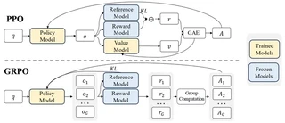
For outcome-level rewards:
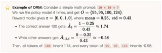
Scoring the group produces rewards $\mathbf r=(r_1,\ldots,r_G)$. Normalize them within the group:
$$ \hat{A}_{i,t}=\hat{r}_i=\frac{r_i-\mathrm{mean}(\mathbf{r})}{\mathrm{std}(\mathbf{r})} $$Each response receives an advantage based on how its reward compares with the group mean, scaled by the group standard deviation. In this outcome-reward formulation, every token in response $i$ shares that advantage. Implementations must also handle zero-variance groups, for example with a small denominator stabilizer.
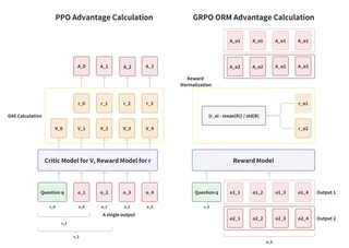
The following worked example illustrates response-level rewards:
A Learning Question: How Can One Advantage Train Every Token?
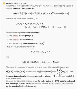
I initially found this confusing: if every token in a response receives the same advantage, how can the model learn which tokens to generate?
In the unclipped score-function term, the shared weight multiplies a different log-probability gradient at every position:
$$ \hat A_i\nabla_\theta\log\pi_\theta(o_{i,t}\mid q,o_{i,\lt t}). $$The weight is response-level, but the gradient depends on the token and its prefix. Different responses receive different weights, so their token sequences contribute differently to the update. Clipping, KL regularization, and shared model parameters also affect the final parameter change.
This provides a learning signal without identifying exactly which token caused the final reward. I find it helpful to distinguish learning from a response-level outcome from having precise token-level credit assignment. They are different claims.
The GRPO Objective and Loss
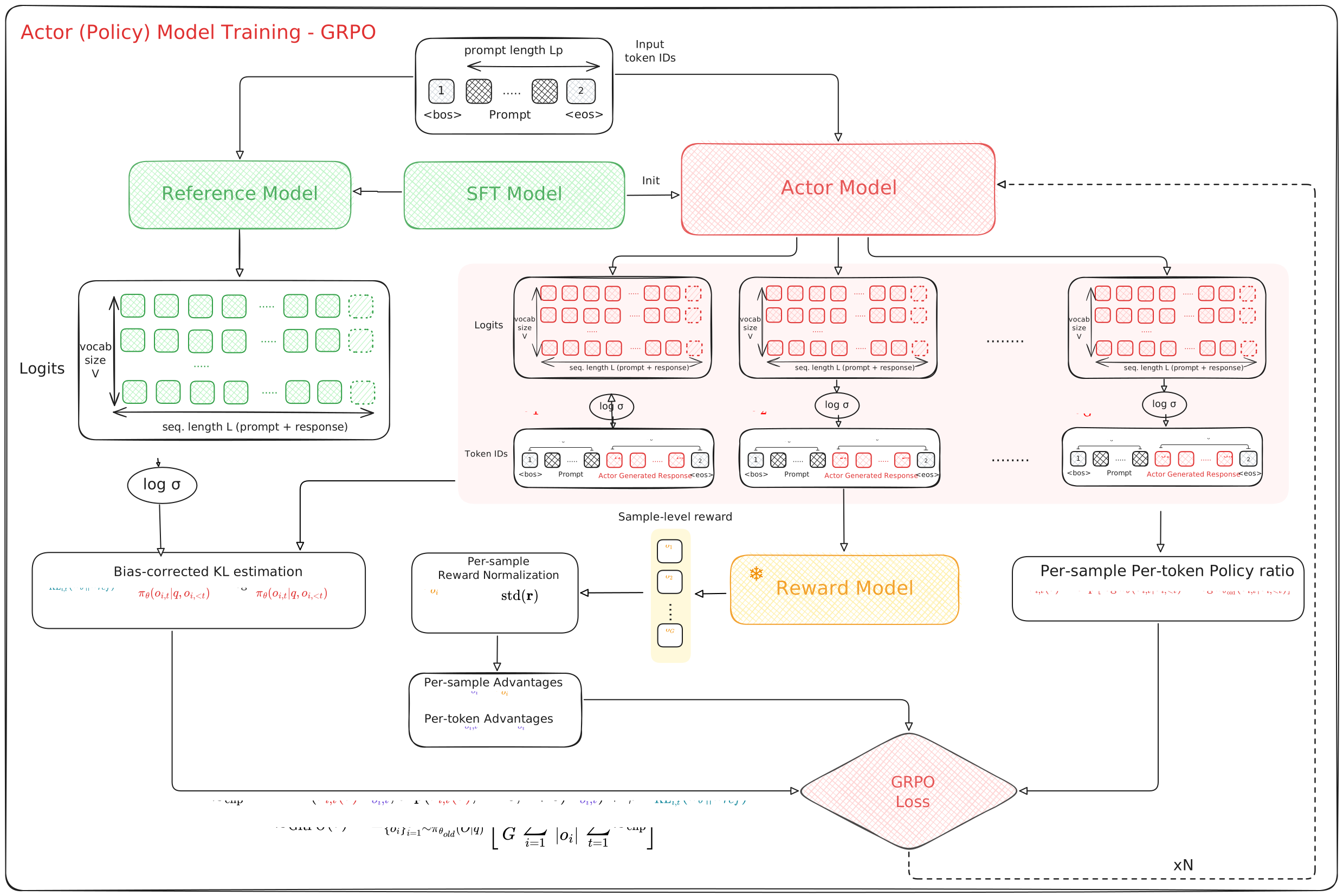
The following loss retains the clipped surrogate, uses group-relative advantages, and adds an explicit KL penalty. It is minimized. First, define
$$ \rho_{i,t}(\theta) =\frac{\pi_\theta(o_{i,t}\mid q,o_{i,\lt t})} {\pi_{\mathrm{old}}(o_{i,t}\mid q,o_{i,\lt t})}. $$The per-token loss is
$$ \begin{aligned} \ell_{i,t}(\theta) ={}&-\min\left( \rho_{i,t}(\theta)\hat A_{i,t}, \operatorname{clip}(\rho_{i,t}(\theta),1-\epsilon,1+\epsilon)\hat A_{i,t} \right)\\ &+\beta k_{i,t}. \end{aligned} $$With prompts $q\sim D$ and response groups sampled from $\pi_{\mathrm{old}}$, average over tokens and responses:
$$ \mathcal{L}_{\mathrm{GRPO}}(\theta) =\mathbb{E}_{q,\{o_i\}_{i=1}^G}\left[ \frac1G\sum_{i=1}^G\frac1{|o_i|}\sum_{t=1}^{|o_i|}\ell_{i,t}(\theta) \right]. $$Here $G$ is the group size, $|o_i|$ is the response length, and $k_{i,t}$ is the KL estimator defined below. This describes the original formulation discussed here; alternative implementations can change the normalization or regularization.
This uses a group-normalized advantage in place of the critic-based estimate and an explicit KL term.
For the sampled token, define $u_{i,t}=\pi_{\mathrm{ref}}(o_{i,t}\mid q,o_{i,\lt t})/\pi_\theta(o_{i,t}\mid q,o_{i,\lt t})$. The KL estimator in this objective is
$$ k_{i,t}=u_{i,t}-\log u_{i,t}-1. $$This expression is nonnegative. Under current-policy sampling and the usual support assumptions, its expectation is $D_{\mathrm{KL}}(\pi_\theta\|\pi_{\mathrm{ref}})$. Rollouts are collected with $\pi_{\mathrm{old}}$, so the sampling distribution matters when describing an estimator as unbiased.
The objective shown here has no separate entropy bonus. Group sampling supplies multiple candidate responses, but should not be treated as mathematically equivalent to an entropy bonus.
Actor Training
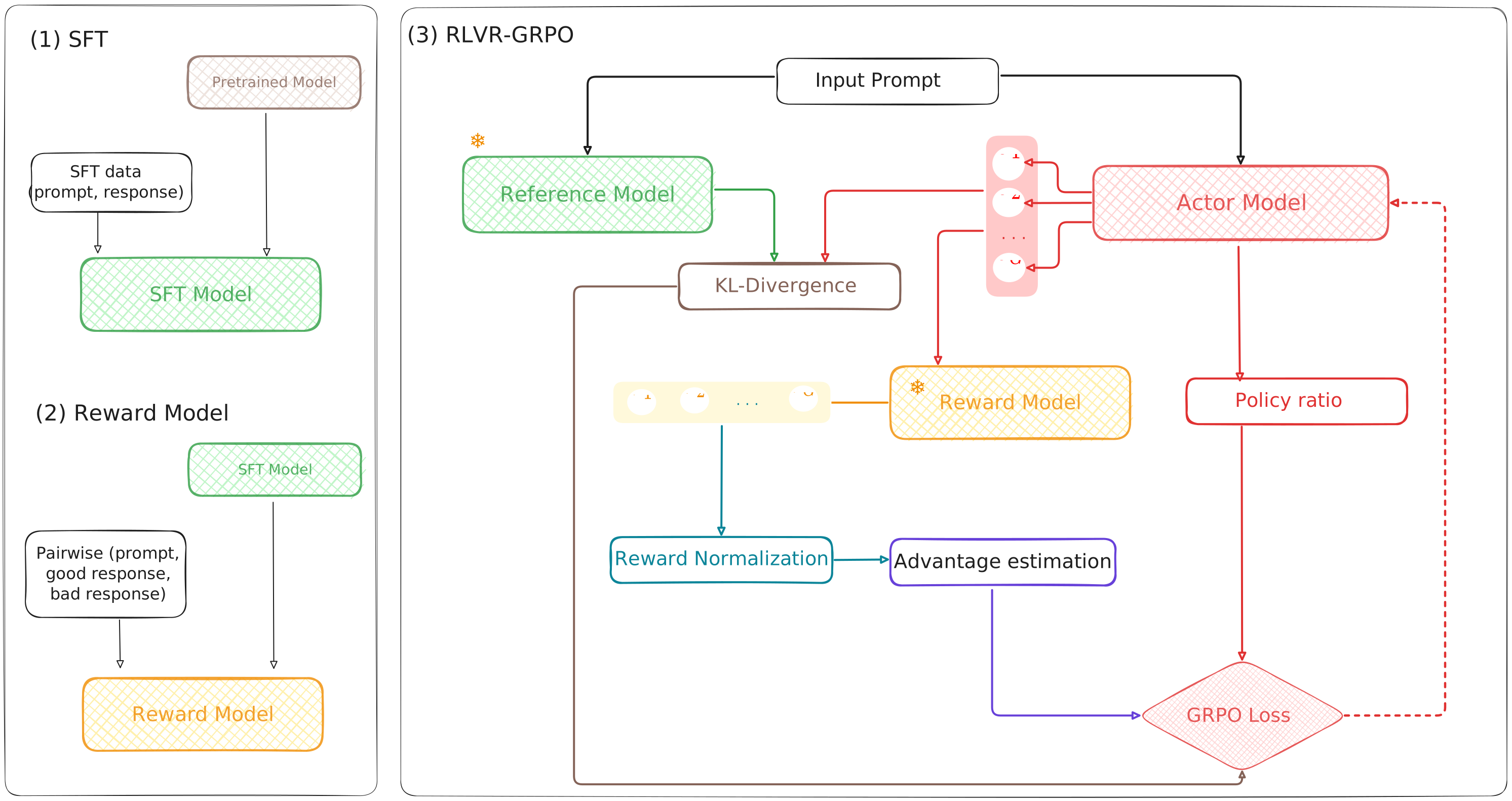
These diagrams connect the GRPO actor update with the overall rollout and optimization loop:
7. PPO and GRPO at a Glance
This comparison refers to the PPO-based RLHF pipeline and the outcome-reward GRPO formulation discussed above.
| Aspect | PPO pipeline | GRPO formulation |
|---|---|---|
| Advantage estimate | Critic-based, commonly using GAE | Relative rewards within a prompt’s response group |
| Learned critic | Used here | Not required |
| Reward signal | Learned or otherwise specified | Learned or verifiable |
| Policy update | Clipped surrogate | Clipped surrogate with group-relative advantages |
| Reference regularization | KL shaping in the reward here | Explicit KL term in the objective shown |
Key Takeaways
- A prompt and response can be viewed as an RL trajectory.
- Preference learning provides a reward signal; policy optimization uses it.
- In PPO-based RLHF, the actor, critic, reward model, and reference policy have distinct roles.
- The rollout policy and the fixed reference policy are different reference points.
- GRPO removes the learned critic by comparing rewards within a response group.
Return to Part 1 for the underlying policy-gradient and PPO derivations.
Acknowledgements
These notes would not have been possible without the many excellent books, lecture notes, blog posts, papers, and open-source resources created by the machine learning community. I am deeply grateful to all of the authors and educators whose work helped me understand reinforcement learning and LLM post-training. Many of the explanations and intuitions presented here were inspired by or built upon these resources, although any mistakes, misunderstandings, or inaccuracies are entirely my own.
If you are interested in learning more, I highly encourage you to explore the references below. They provide much deeper and more rigorous treatments than these personal notes and have been invaluable throughout my learning journey.
References
RL Foundations
Policy Gradient Papers
Sutton et al. — Policy Gradient Methods for Reinforcement Learning with Function Approximation
Mnih et al. — Asynchronous Methods for Deep Reinforcement Learning
RLHF
Christiano et al. — Deep Reinforcement Learning from Human Preferences
Ouyang et al. — Training Language Models to Follow Instructions with Human Feedback
Ziegler et al. — Fine-Tuning Language Models from Human Preferences
PPO and GRPO Explanations

Hi! I’m Chi, and I am interested in developing multimodal AI systems that can meaningfully improve medical understanding and support clinical decision-making.
My research lies at the intersection of machine learning and medical imaging, with a particular focus on multimodal foundation models, medical reasoning, and trustworthy AI for healthcare. I am especially interested in building clinically grounded and reliable models that can learn from complex medical data while remaining interpretable and useful in real-world settings.
During my research journey, I have been fortunate to work under the guidance of Prof. Yueming Jin at the National University of Singapore, Prof. Lee Hwee Kuan at the Bioinformatics Institute (A*STAR), Prof. Hieu Pham at VinUniversity, and Prof. Ravishankar K. Iyer at the University of Illinois Urbana–Champaign. Feel free to reach out if you would like to chat about medical AI, multimodal learning, or research in general!